基于3D颗粒的流体模拟

Contribution (Alphabeta): Jiannan jiang, Shixuan Li, Yifei Xing Video Report: Link for Video PPT Slides: Link for Slides

Abstract

Fluid dynamics requires costly rendering and simulation. In this project we treat fluids as a set of particles moving at various velocities. The rendering of each particle consists internal and external forces, bounces, and viscosity. The inspirations for the algorithms updating the attributes and positions of each particle comes from the paper Position Based Fluids. The starter code system implements the nanogui system from Project 4 [Cloth Simulator].

Implementation

Overview

There are two components of our system. The first component is a continuously rendering system which iterates through the particles and updates the velocity, forces, and position attributes. The calculation steps consists of an analysis of constraints based on neighboring particles. The second component is the interaction module which handles the mouse and keyboard movement also with an GUI presentation which allows user to change environment and particle features and exert manual changes and interactions.

Fluid Dynamics

There is a sequence of constraints to be updated in each iteration. The steps are shown below: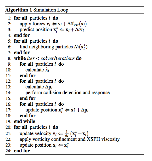

External Forces

The first step is to accumulate the external forces and perform the first-step prediction for the position of the particles based on its velocity. In this project, the only natural constant force to be applied is the gravity. Thus, we firstly just apply the gravity forces on each particle and get the velocity and thus position updates. The velocity is calculated using the simple kinematics physics equations with general idea of Euler's Method, where t is a very small time delta which depends on the number of steps and frames per second of rendering: \(t = \frac{1}{m[frames/sec] * n[steps/frame]}\) \(v = v_0 + at\) From the velocity, we can use a similar equation to find the predicted position: \(p = p_0 + vt\)

Finding Neighbors

To determine the forces between particles, we need to find the neighboring particles first. The idea is to select according to a bounding sphere centered with the particle and filter out neighboring particles by position.

Particle Forces

Incompressibility

The calculation of force is based on a particle's position and its neighbors. The idea is to create a density field which decides the overall forces exerted on the particle. The idea is that the fluid must maintain a constant density. To do this, we must make sure that the position of each particle in every iteration makes the particle's density as close to the rest density as possible. Thus, the first step would be to calculate the density of each particle. This is done by using the SPH (Smoothed Particle Hydro-dynamic) density estimation standard. W represents a kernel and h is the cut-off distance for a particle's neighbor. \(\sum_{j}W(p_i - p_j , h)\)

The kernel we use here is Poly6 Kernel, as with Müller et al

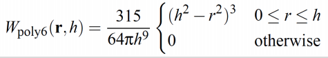
The estimation process is basically summing up the difference in positions between a particle and its neighbors, weighted by a kernel.

The dencity constraint on the ith paricle is defined using an equation of state: \(C_i (p_1 ,\ldots, p_n) = \frac{\rho_i}{\rho_0} -1\) where \(\rho_0\) is the rest density and \(\rho_i\) is given by the standard SPH estimator: \(\rho_i = \sum_{j} m_j W(p_i - p_j , h)\) The Position Based Dynamics method finds a particle position correction \(\Delta p\) that satisfies the constraint: \(C(p + \Delta p) = 0\) We can find it by a series of Newton's Method along the constraint gradient: \(\Delta p \approx \nabla C(p)\lambda\) \(C(p+\Delta p) \approx C(p) + \nabla C^{T} \Delta p = C(p) + \nabla C^{T}\nabla C \lambda = 0\)

The gradient of a constraint is defined as following: 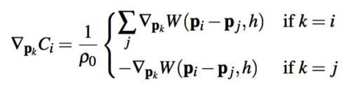The kernel used here is the Spiky Kernel:

Plugging this into our approximation, we can solve for lambda as the following. Note that the \(\epsilon\) appeared in the denominator is a method we use to regularize the constraint using constraint force mixing. This is because otherwise the original denominator \(\sum_{k}|\nabla_{p_k}C_i|^{2}\) will become unstable when particles are close to separating. Thus, we can improve the accuracy by adding a relaxation parameter to the diagonal of the parameter matrix. \(\lambda_i = - \frac{C_i (p_1 ,\ldots ,p_n)}{\sum_{k}|\nabla_{p_k}C_i|^{2} + \epsilon}\) Thus, the final position update for particle i is: \(\lambda p_i = \frac{1}{\rho_0} \sum_{j} (\lambda_i + \lambda_j) \nabla W(p_i - p_j , h)\)

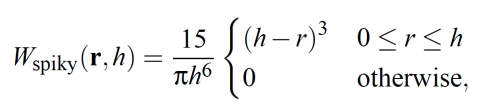
With such method, we can update each particle's position in every iteration.

Tensile Instability

When a particle has too few neighbor, it may end up taking negative pressure and clump together. Thus, in order to repulse the particles, we need add the surface tension, an artificial pressure, to the smoothing kernel. The corrective term is described by Monaghan, and is then added to our position update: \(s_{corr} = -k(\frac{W(p_i - p_j , h)}{W(\Delta q, h)})^n\) \(\Delta p_i = \frac{1}{\rho_0}\sum_{j}(\lambda_i + \lambda_j + s_{corr})\nabla W(p_i - p_j , h)\)

The \(\Delta q\) is a fraction of our neighbor cut-off distance (\(h\)), and the k and n are small constants. Here we use \(k = 0.001\), \(n = 4\), and \(\Delta q = 0.01 * h\), which are all tested values that made the simulation look most nature by experience.

Viscosity

In order to confine some unnatural oscillations and make the set of particles more fluid-like, we apply some slight damping by introducing viscosity to the fluid. The viscosity of a fluid describes the thickness and stickiness of a fluid. The update of each particle's velocity is based on the following equation: \(v_{i}^{new} = v_i + c \sum_{j} v_{ij} W(p_i - p_j , h)\)

Rendering Structure

The overall structure of our simulation loop consists the following steps: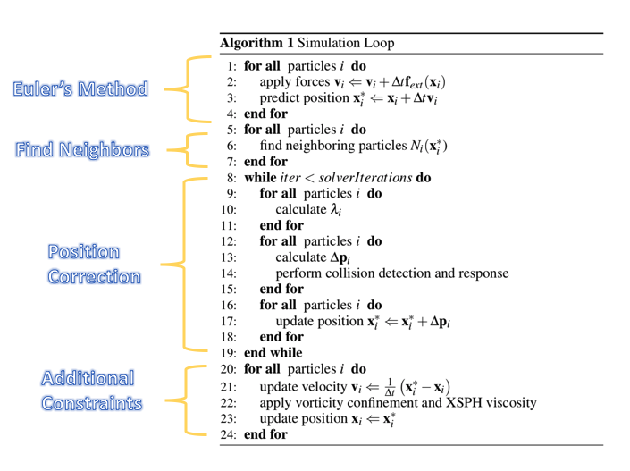

Final Result

Simulation Loop

Interaction

Showing a single model of water flow may not show the full attribute of the fluid. Thus, in order to create more testing models and make it more fun, we developed some interaction methods which allows the user to exert more control to the system.

Water Drop

In our user interface, we have a button enabling additional drops of particles. Once turned on, the dropping methods allows the user to add 3x3x3 particle drops to the fluid by clicking.

Concentration

The original system is basically operating under a single natural force: gravity. This successfully mimics the real-life situation, but also limits the functionalities of the system. Thus, we decided to allow users to add more artificial forces to the system, which we call the "concentration" in out interaction method. The concentration method allows the user to "drag" the fluid particles with the mouse. In other words, the particles will "concentrate" on the mouse's movement. The concentration is realized by calculating the force from the mouse to each particles according to their distance. The closer to the mouse, the stronger the force. There is also a parameter called "concentration intensity" which represents the force intensity for each particle to concentrate on the mouse. The user can change this parameter on the user interface. With concentration, we can create much more fun!

Concentration Intensity = 10

Concentration Intensity = 100

Lessons Learned

In this project, we strive to achieve a real-time realistic rendering of fluids. However, the term "realistic" is always vaguer than it sounds. When implementing the fluid dynamics with SPH methods, we made some test cases with correct implementation but did not get a satisfying result as particles are going the other way around (violates our intuition). Therefore, we made a hack and let the particles go the other way, which does not cause much issue as then our fluid looks fine when settled. Then, when comparing our result with other fluid simulation results, we found that our fluid are not behaving well that individual particles are not attracting each other to form a nice fluid surface in a cohesive manner. Particularly, our fluid expands in the first few frames. We are well aware of this and implemented fluids with correct sign. However, in the newer version we require quite a lot particles ( at least thousands of particles) to make the simulation looks nice. Given our computation powers, the rendering is no longer real-time and hugely deviates from our original intention, as we have added direct manipulation and real time interaction of the fluid. Our team members have discussed this and decide to leave both version as we presented in the presentation to allow more fluent and more interactive setting. As such, we learned how tricky it can be when dealing with physical models when using test case of small size, how hard to achieve realism in simulation, , and the tradeoff between availability and correctness.

Reference

• Miles Macklin and Matthias Müller. Position based fluids. ACM Trans.Graph., 32(4):104:1–104:12, July 2013.
• Matthias Müller, David Charypar and Markus Gross. Particle-Based Fluid Simulation for Interactive Applications. Eurographics/SIGGRAPH Symposium on Computer Animation (2003)
• J. J. Monaghan. Smoothed Particle Hydrodynamics. Department of Mathematics, Monash University, Clayton, Victoria 316 8, Australia
• Kenneth Bodin, Claude Lacoursie`re, and Martin Servin. Constraint Fluids. IEEE Transactions on Visualization and Computer Graphics, Vol. 18, NO. 3, March 2012